Manejo de datos raster
Contents
Manejo de datos raster#
Descripción general#
En este capítulo, se muestran ejemplos de manejo de datos raster con Python.
Los datos se obtienen de servicios basados en la especificación SpatioTemporal Asset Catalogs (STAC), la cual proporciona una estructura común para describir y catalogar recursos espacio temporales (ej. imágenes satelitales) a través de una interfaz de programación de aplicaciones (en inglés, API o Application Programming Interface). Puede explorar catálogos y API de tipo STAC en el sitio web STAC browser.
Instalación de módulos#
Algunos de los módulos que se utilizan en este capítulo son:
rasterio: para operaciones generales de manejo de datos raster.
xarray: para manejo de arreglos multidimensionales.
rioxarray: extensión de xarray para trabajar con rasterio.
pystac_client: para trabajar con catálogos STAC.
# Instalación, mediante mamba, de módulos para manejo de datos raster y acceso a recursos STAC
mamba install -c conda-forge xarray rioxarray earthpy xarray-spatial pystac-client python-graphviz
Lectura#
Acceso a recursos STAC#
# Carga de pystac_client, para acceder datos en STAC
from pystac_client import Client
Se accede el API de Earth Search, el cual proporciona acceso a conjuntos de datos públicos en Amazon Web Services (AWS).
La función Client.open() retorna un objeto tipo Client, el cual se utiliza para acceder el API (ej. realizar búsquedas).
# URL del API STAC
api_url = "https://earth-search.aws.element84.com/v0"

# Cliente para acceso a los datos
client = Client.open(api_url)
En este ejemplo, se accederá una colección de imágenes Sentinel en formato Cloud Optimized GeoTIFF (COG).
# Colección
collection = "sentinel-s2-l2a-cogs"
Se especifica un punto (x, y) para buscar imágenes que lo contengan.
# Punto para búsqueda
from shapely.geometry import Point
point = Point(-84, 10)
La función Client.search() realiza una búsqueda con base en criterios como colección e intersección.
# Búsqueda de items (imágenes) que contienen el punto
search = client.search(collections=[collection],
                       intersects=point,
                       max_items=10,
)
# Cantidad total de items que retorna la búsqueda
search.matched()
370
# Items retornados
items = search.get_all_items()

len(items)
10
# Identificadores de los items retornados
for item in items:
    print(item)
<Item id=S2A_16PHS_20221126_0_L2A>
<Item id=S2B_16PHS_20221121_0_L2A>
<Item id=S2A_16PHS_20221116_0_L2A>
<Item id=S2B_16PHS_20221111_0_L2A>
<Item id=S2A_16PHS_20221106_0_L2A>
<Item id=S2B_16PHS_20221101_0_L2A>
<Item id=S2A_16PHS_20221027_0_L2A>
<Item id=S2B_16PHS_20221022_0_L2A>
<Item id=S2A_16PHS_20221017_0_L2A>
<Item id=S2B_16PHS_20221012_0_L2A>
Para estudiarlo en detalle, se selecciona un item.
# Primer item (imagen) retornado
item = items[0]
Nótese que al seleccionarse el item mediante una posición en una colección, la imagen correspondiente puede cambiar si se actualizan los datos del API.
# Algunos atributos del item
print(item.id)
print(item.datetime)
print(item.geometry)
print(item.properties)
S2A_16PHS_20221126_0_L2A
2022-11-26 16:10:31+00:00
{'type': 'Polygon', 'coordinates': [[[-83.26529071959975, 9.841749072035094], [-84.26505426889273, 9.85133238997552], [-84.2564449365329, 10.843245515578994], [-83.25354975084628, 10.83267581874028], [-83.26529071959975, 9.841749072035094]]]}
{'datetime': '2022-11-26T16:10:31Z', 'platform': 'sentinel-2a', 'constellation': 'sentinel-2', 'instruments': ['msi'], 'gsd': 10, 'view:off_nadir': 0, 'proj:epsg': 32616, 'sentinel:utm_zone': 16, 'sentinel:latitude_band': 'P', 'sentinel:grid_square': 'HS', 'sentinel:sequence': '0', 'sentinel:product_id': 'S2A_MSIL2A_20221126T160511_N0400_R054_T16PHS_20221126T205802', 'sentinel:data_coverage': 100, 'eo:cloud_cover': 77.02, 'sentinel:valid_cloud_cover': True, 'sentinel:processing_baseline': '04.00', 'sentinel:boa_offset_applied': True, 'created': '2022-11-26T23:45:01.332Z', 'updated': '2022-11-26T23:45:01.332Z'}
Ahora, se realiza la búsqueda con base en un rectángulo delimitador (bounding box) generado a partir del punto que se definió anteriormente.
# Rectángulo para búsquedas
bbox = point.buffer(0.01).bounds
bbox
(-84.01, 9.99, -83.99, 10.01)
También se restringe la búsqueda para retornar solo aquellas imágenes con cobertura de nubes menor al 10%.
# Búsqueda con nuevos criterios
search = client.search(collections=[collection],
                       bbox=bbox,
                       datetime="2022-01-01/2022-10-30",
                       query=["eo:cloud_cover<10"]) # no deben haber espacios alrededor del '<'

# Cantidad total de items que retorna la búsqueda
search.matched()
5
# Items retornados
items = search.get_all_items()

len(items)
5
# Segundo item retornado y algunos de sus atributos
item = items[1]

print(item.datetime)
print(item.properties)
2022-06-04 16:10:32+00:00
{'datetime': '2022-06-04T16:10:32Z', 'platform': 'sentinel-2b', 'constellation': 'sentinel-2', 'instruments': ['msi'], 'gsd': 10, 'view:off_nadir': 0, 'proj:epsg': 32616, 'sentinel:utm_zone': 16, 'sentinel:latitude_band': 'P', 'sentinel:grid_square': 'HS', 'sentinel:sequence': '0', 'sentinel:product_id': 'S2B_MSIL2A_20220604T160509_N0400_R054_T16PHS_20220604T202130', 'sentinel:data_coverage': 100, 'eo:cloud_cover': 5.33, 'sentinel:valid_cloud_cover': True, 'sentinel:processing_baseline': '04.00', 'sentinel:boa_offset_applied': True, 'created': '2022-06-05T01:47:01.875Z', 'updated': '2022-06-05T01:47:01.875Z'}
Ejercicio#
Realice el ejercicio de búsqueda de imágenes Landsat 8 del curso The Carpentries Incubator - Introduction to Geospatial Raster and Vector Data with Python. Puede cambiar el punto de la búsqueda por otro que sea de su interés.
Assets#
Cada item retornado contiene un conjunto de “activos” (assets) (ej. bandas) que también pueden accederse mediante el API.
# Activos (assets) del item
assets = item.assets

# Llaves
assets.keys()
dict_keys(['thumbnail', 'overview', 'info', 'metadata', 'visual', 'B01', 'B02', 'B03', 'B04', 'B05', 'B06', 'B07', 'B08', 'B8A', 'B09', 'B11', 'B12', 'AOT', 'WVP', 'SCL'])
# Contenido completo de los items
assets.items()
dict_items([('thumbnail', <Asset href=https://roda.sentinel-hub.com/sentinel-s2-l1c/tiles/16/P/HS/2022/6/4/0/preview.jpg>), ('overview', <Asset href=https://sentinel-cogs.s3.us-west-2.amazonaws.com/sentinel-s2-l2a-cogs/16/P/HS/2022/6/S2B_16PHS_20220604_0_L2A/L2A_PVI.tif>), ('info', <Asset href=https://roda.sentinel-hub.com/sentinel-s2-l2a/tiles/16/P/HS/2022/6/4/0/tileInfo.json>), ('metadata', <Asset href=https://roda.sentinel-hub.com/sentinel-s2-l2a/tiles/16/P/HS/2022/6/4/0/metadata.xml>), ('visual', <Asset href=https://sentinel-cogs.s3.us-west-2.amazonaws.com/sentinel-s2-l2a-cogs/16/P/HS/2022/6/S2B_16PHS_20220604_0_L2A/TCI.tif>), ('B01', <Asset href=https://sentinel-cogs.s3.us-west-2.amazonaws.com/sentinel-s2-l2a-cogs/16/P/HS/2022/6/S2B_16PHS_20220604_0_L2A/B01.tif>), ('B02', <Asset href=https://sentinel-cogs.s3.us-west-2.amazonaws.com/sentinel-s2-l2a-cogs/16/P/HS/2022/6/S2B_16PHS_20220604_0_L2A/B02.tif>), ('B03', <Asset href=https://sentinel-cogs.s3.us-west-2.amazonaws.com/sentinel-s2-l2a-cogs/16/P/HS/2022/6/S2B_16PHS_20220604_0_L2A/B03.tif>), ('B04', <Asset href=https://sentinel-cogs.s3.us-west-2.amazonaws.com/sentinel-s2-l2a-cogs/16/P/HS/2022/6/S2B_16PHS_20220604_0_L2A/B04.tif>), ('B05', <Asset href=https://sentinel-cogs.s3.us-west-2.amazonaws.com/sentinel-s2-l2a-cogs/16/P/HS/2022/6/S2B_16PHS_20220604_0_L2A/B05.tif>), ('B06', <Asset href=https://sentinel-cogs.s3.us-west-2.amazonaws.com/sentinel-s2-l2a-cogs/16/P/HS/2022/6/S2B_16PHS_20220604_0_L2A/B06.tif>), ('B07', <Asset href=https://sentinel-cogs.s3.us-west-2.amazonaws.com/sentinel-s2-l2a-cogs/16/P/HS/2022/6/S2B_16PHS_20220604_0_L2A/B07.tif>), ('B08', <Asset href=https://sentinel-cogs.s3.us-west-2.amazonaws.com/sentinel-s2-l2a-cogs/16/P/HS/2022/6/S2B_16PHS_20220604_0_L2A/B08.tif>), ('B8A', <Asset href=https://sentinel-cogs.s3.us-west-2.amazonaws.com/sentinel-s2-l2a-cogs/16/P/HS/2022/6/S2B_16PHS_20220604_0_L2A/B8A.tif>), ('B09', <Asset href=https://sentinel-cogs.s3.us-west-2.amazonaws.com/sentinel-s2-l2a-cogs/16/P/HS/2022/6/S2B_16PHS_20220604_0_L2A/B09.tif>), ('B11', <Asset href=https://sentinel-cogs.s3.us-west-2.amazonaws.com/sentinel-s2-l2a-cogs/16/P/HS/2022/6/S2B_16PHS_20220604_0_L2A/B11.tif>), ('B12', <Asset href=https://sentinel-cogs.s3.us-west-2.amazonaws.com/sentinel-s2-l2a-cogs/16/P/HS/2022/6/S2B_16PHS_20220604_0_L2A/B12.tif>), ('AOT', <Asset href=https://sentinel-cogs.s3.us-west-2.amazonaws.com/sentinel-s2-l2a-cogs/16/P/HS/2022/6/S2B_16PHS_20220604_0_L2A/AOT.tif>), ('WVP', <Asset href=https://sentinel-cogs.s3.us-west-2.amazonaws.com/sentinel-s2-l2a-cogs/16/P/HS/2022/6/S2B_16PHS_20220604_0_L2A/WVP.tif>), ('SCL', <Asset href=https://sentinel-cogs.s3.us-west-2.amazonaws.com/sentinel-s2-l2a-cogs/16/P/HS/2022/6/S2B_16PHS_20220604_0_L2A/SCL.tif>)])
# Nombres de los activos
for key, asset in assets.items():
    print(f"{key}: {asset.title}")
thumbnail: Thumbnail
overview: True color image
info: Original JSON metadata
metadata: Original XML metadata
visual: True color image
B01: Band 1 (coastal)
B02: Band 2 (blue)
B03: Band 3 (green)
B04: Band 4 (red)
B05: Band 5
B06: Band 6
B07: Band 7
B08: Band 8 (nir)
B8A: Band 8A
B09: Band 9
B11: Band 11 (swir16)
B12: Band 12 (swir22)
AOT: Aerosol Optical Thickness (AOT)
WVP: Water Vapour (WVP)
SCL: Scene Classification Map (SCL)
# Imagen thumbnail
assets["thumbnail"]
Asset: Thumbnail
| href: https://roda.sentinel-hub.com/sentinel-s2-l1c/tiles/16/P/HS/2022/6/4/0/preview.jpg |
| Title: Thumbnail |
| Media type: image/png |
| Roles: ['thumbnail'] |
| Owner: |
# URL del thumbnail
assets["thumbnail"].href
'https://roda.sentinel-hub.com/sentinel-s2-l1c/tiles/16/P/HS/2022/6/4/0/preview.jpg'
Visualización#
# Carga de rioxarray, para graficar datos raster
import rioxarray
El módulo rioxarray provee un conjunto de funciones para manipular imágenes.
Las bandas pueden abrirse con la función open_rasterio() y graficarse con plot() y plot.imshow().
Visualización del overview#
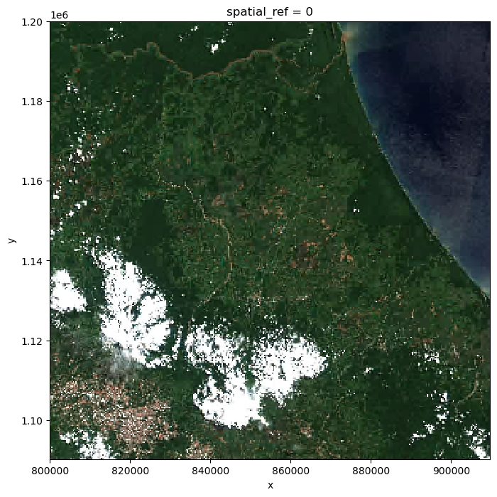
El overview es una imagen de tres bandas tipo “True Color”.
# Vista general de la imagen (True Color)
overview = rioxarray.open_rasterio(item.assets['overview'].href)

overview
<xarray.DataArray (band: 3, y: 343, x: 343)>
[352947 values with dtype=uint8]
Coordinates:
  * band         (band) int64 1 2 3
  * x            (x) float64 8.001e+05 8.005e+05 ... 9.093e+05 9.096e+05
  * y            (y) float64 1.2e+06 1.2e+06 1.199e+06 ... 1.091e+06 1.09e+06
    spatial_ref  int64 0
Attributes:
    AREA_OR_POINT:       Area
    OVR_RESAMPLING_ALG:  AVERAGE
    _FillValue:          0
    scale_factor:        1.0
add_offset: 0.0# Dimensiones de la imagen (bandas, filas, columnas)
overview.shape
(3, 343, 343)
# Graficación de imagen RGB
overview.plot.imshow(figsize=(8, 8))
<matplotlib.image.AxesImage at 0x7fcaae8b67a0>
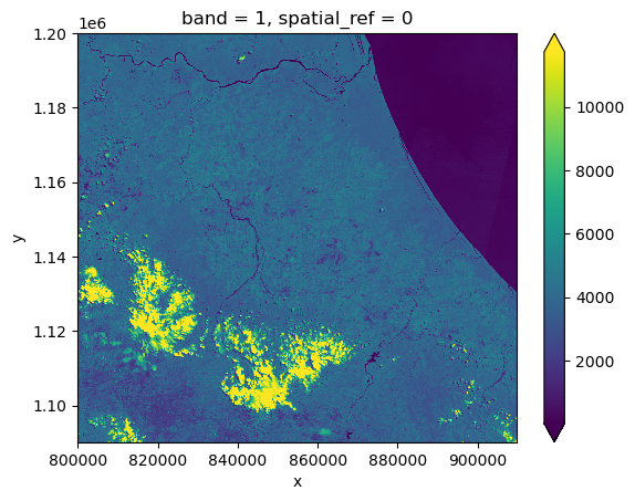
Visualización de una banda#
# Banda 9
b_09 = rioxarray.open_rasterio(assets["B09"].href)

b_09
<xarray.DataArray (band: 1, y: 1830, x: 1830)>
[3348900 values with dtype=uint16]
Coordinates:
  * band         (band) int64 1
  * x            (x) float64 8e+05 8.001e+05 8.001e+05 ... 9.097e+05 9.098e+05
  * y            (y) float64 1.2e+06 1.2e+06 1.2e+06 ... 1.09e+06 1.09e+06
    spatial_ref  int64 0
Attributes:
    AREA_OR_POINT:       Area
    OVR_RESAMPLING_ALG:  AVERAGE
    _FillValue:          0
    scale_factor:        1.0
add_offset: 0.0# Graficación de la banda
# robust=True calcula el rango de colores entre los percentiles 2 y 98
b_09.plot(robust=True)
<matplotlib.collections.QuadMesh at 0x7fcaae5f1bd0>
Ejemplo de álgebra raster: cálculo del NDVI#
Seguidamente, se utiliza la imagen Sentinel para calcular el Índice de vegetación de diferencia normalizada (NDVI).
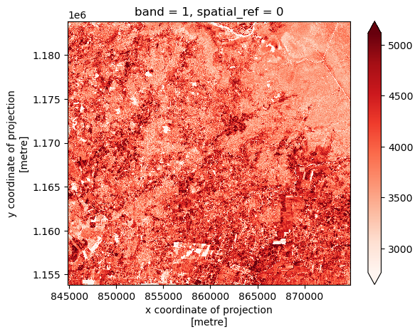
Se separan las dos bandas necesarias para el cálculo: la roja y la infrarroja cercana.
# Bandas necesarias para el cálculo
b_red = rioxarray.open_rasterio(assets["B04"].href)
b_nir = rioxarray.open_rasterio(assets["B8A"].href)
Para efectos del ejemplo, se reduce el área en la que va a realizarse el cálculo.
# Buffer (rectángulo) de 15 km alrededor de un punto
point = Point(859872, 1168852)
bbox = point.buffer(15000).bounds

# Recorte
b_red_clip = b_red.rio.clip_box(*bbox)
b_nir_clip = b_nir.rio.clip_box(*bbox)
# Visualización de la banda roja
b_red_clip.plot(robust=True, cmap="Reds")
# Visualización de la banda infrarroja cercana
b_nir_clip.plot(robust=True, cmap="Reds")
<matplotlib.collections.QuadMesh at 0x7efe03da5330>
# Dimensiones de las bandas
print(b_red_clip.shape, b_nir_clip.shape)
(1, 3001, 3001) (1, 1501, 1501)
Para realizar la operación algebraica, las bandas deben tener las mismas dimensiones. Así que se reduce la resolución de la banda roja para hacerla igual a la resolución de la infrarroja cercana.
# Se homogeneizan las dimensiones
b_red_clip_matched = b_red_clip.rio.reproject_match(b_nir_clip)
print(b_red_clip_matched.shape)
(1, 1501, 1501)
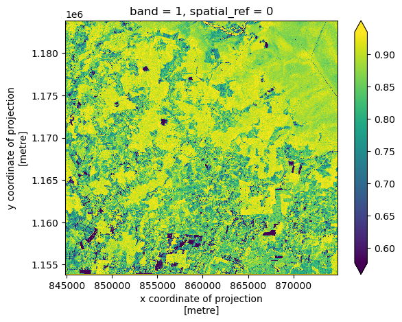
Ya puede calcularse el NDVI.
# Cálculo del NDVI
ndvi = (b_nir_clip - b_red_clip_matched)/ (b_nir_clip + b_red_clip_matched)
# Visualización del cálculo del NDVI
ndvi.plot(robust=True)
<matplotlib.collections.QuadMesh at 0x7efe007cc790>
Escritura#
La función to_raster() exporta los datos a un archivo raster.
# Se guarda el resultado del cálculo del NDVI en un archivo
# ndvi.rio.to_raster("ndvi.tif")